Tip of the Week: Add Dropdown Menus to Your Excel Spreadsheets

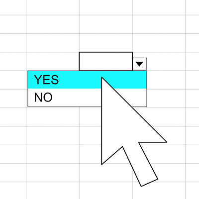
If you know how to use functions and various other features that Microsoft Excel and Google Sheets have to offer, then you can take your skills one step further than most. One such feature is the use of dropdown menus within cells. Let’s discuss how you can use them to your benefit in both Excel and Sheets.

Create Your First Dropdown Menu in Excel

The first step to making your dropdown is to create the list it’s based off of. On your Excel sheet, create a new table that contains the options you want to include with your dropdown. Once you have done this, you can select a cell to house your dropdown menu.

Once you have selected your cell, you must navigate to the Ribbon to find the Data tab. Select the Data Validation option. Once you do this, you go to the Settings tab and select List from the Allow box.

In the Source box, you need to select the data range that is populated by the table you have just created. Be sure to omit the cell that contains the title. If you want it to be okay if the user leaves the dropdown blank, you can select the Ignore Blank box to make sure it’s checked. While you’re here, make sure In-Cell Dropdown is checked as well.

Under the Input Message tab, you can have your cell display a message when it is selected. This is done through the use of the Show input message when cell is selected box. You then provide a title and a message to display.

Under the Error Alert tab, you can have the software notify the user when they have entered something that isn’t included in the list. Check the Show error alert after invalid data is entered box, after which you’ll be prompted to enter a title and message to display. You can also style the alert here.

• Information or Warning won’t stop someone from putting data not included in the list in, and will display a blue circle with an “I” in it or the yellow warning triangle respectively.
• Stop will prevent someone from entering data not included in your list at all.

Build a Dropdown Menu in Google Sheets

Google Sheets also makes it easy for you to build a dropdown menu. To get started, you have to determine if you want to use specific words or numbers. If you do, then select the cell or range of cells you want to use for your dropdown. Select Data from the toolbar, then select Data Validation. On this panel, you can select List from a Range to define the Criteria. From the menu, select List of Items.

In the box next to your selection, you can type out the options you want to display on the list, separated by commas (but no spaces). For instance: banana,orange,apple,grape

You should see a small downward arrow appear by default in the cells used for the dropdown. You can disable this feature through the Show dropdown list in cell option. Once you’re done, click Save.

If you want to use data already found in the spreadsheet, you can do this as well. Select the range of cells you want to populate your list with. Select Data > Data Validation, and leave Criteria set to List from a Range. Input the range of cells that you want to use for your list. For example, if your list ranges from F5 to F12, type in F5:F12. You’ll see a small grid pattern appear in the entry box so you can manually select which cells you want to include. Once you’re done, click Save.

We hope you find this tip helpful for organizing your data. If you would like additional support, be sure to contact Microtechs at (415) 246-0101.